Photo by Stephen Phillips - Hostreviews.co.uk on UnSplash
In Part 4, we looked into some crucial sample pre-processing steps before modeling, establishing the required pipeline for data processing, evaluating various algorithms, and ultimately identifying an appropriate baseline model, that is CatBoost. As we proceed to Part 5, our focus will be on assessing the significance of features in the initial scraped dataset. We’ll achieve this by employing the feature_importances_ method of CatBoostRegressor and analyzing SHAP values. Additionally, we’ll systematically eliminate features showing lower importance or predictive capability. Excited to delve into this phase!
Our initial step involves executing a train-test split. This process divides the data into two distinct sets: a training set and a testing set. The training set is employed for model training, while the testing set is exclusively reserved for model evaluation. This methodology allows models to be trained on the training set and then assessed for accuracy using the unseen testing set. Ultimately, this approach enables an unbiased evaluation of our model’s performance, utilizing the test set that remained untouched during the model training phase.
Code
train, test = model_selection.train_test_split( df, test_size=0.2, random_state=utils.Configuration.seed)print(f"Shape of train: {train.shape}")print(f"Shape of test: {test.shape}")
Shape of train: (2928, 56)
Shape of test: (732, 56)
Preprocess dataframe for modelling
Our first step entails removing features that lack informative value for our model, including ‘external_reference’, ‘ad_url’, ‘day_of_retrieval’, ‘website’, ‘reference_number_of_the_epc_report’, and ‘housenumber’. After this, we’ll proceed to apply a log transformation to our target variable. Furthermore, we’ll address missing values in categorical features by replacing them with the label “missing value.” This step is crucial as CatBoost can handle missing values in numerical columns, but for categorical missing values, user intervention is needed.
Code
processed_train = ( train.reset_index(drop=True) .assign(price=lambda df: np.log10(df.price)) # Log transformation of 'price' column .drop(columns=utils.Configuration.features_to_drop))# This step is needed since catboost cannot handle missing values when feature is categoricalfor col in processed_train.columns:if processed_train[col].dtype.name in ("bool", "object", "category"): processed_train[col] = processed_train[col].fillna("missing value")processed_train.shape
(2928, 50)
Inspect feature importance
To evaluate feature importance, we’re utilizing two methods: the feature_importances_ attribute in CatBoost and SHAP values from the SHAP library. To begin examining feature importances, we’ll initiate model training. This involves further partitioning the training set, reserving a portion for CatBoost training (validation dataset). This segmentation allows us to stop the training process when overfitting emerges. Preventing overfitting is crucial, as it ensures we don’t work with an overly biased model. Additionally, if overfitting occurs, stopping training earlier helps conserve time and resources.
As you can see below, the training loss steadily decreases, but the validation loss reaches a plateau. Thanks to the validation dataset, we can halt the training well before the initially set 2000 iterations. This early cessation is crucial for preventing overfitting and ensures a more balanced and effective model.
Learning rate set to 0.038132
0:  learn: 0.3187437    test: 0.3148628 best: 0.3148628 (0) total: 186ms    remaining: 6m 12s
Stopped by overfitting detector  (20 iterations wait)

bestTest = 0.1087393065
bestIteration = 850

Shrink model to first 851 iterations.
<catboost.core.CatBoostRegressor at 0x240921b25c0>
According to our trained CatBoost model, the most significant feature in our dataset is the living_area, followed by cadastre_income and latitude. To validate and compare these findings, we’ll examine the SHAP values to understand how they align or differ from the feature importances provided by the model.
SHAP (SHapley Additive exPlanations) values offer a method to elucidate the predictions made by any machine learning model. These values leverage a game-theoretic approach to quantify the contribution of each “player” (feature) to the final prediction. In the realm of machine learning, SHAP values assign an importance value to each feature, delineating its contribution to the model’s output.
SHAP values provide detailed insights into how each feature influences individual predictions, their relative significance in comparison to one another, and the model’s reliance on interactions between features. This comprehensive perspective enables a deeper understanding of the factors that drive the model’s decision-making process.
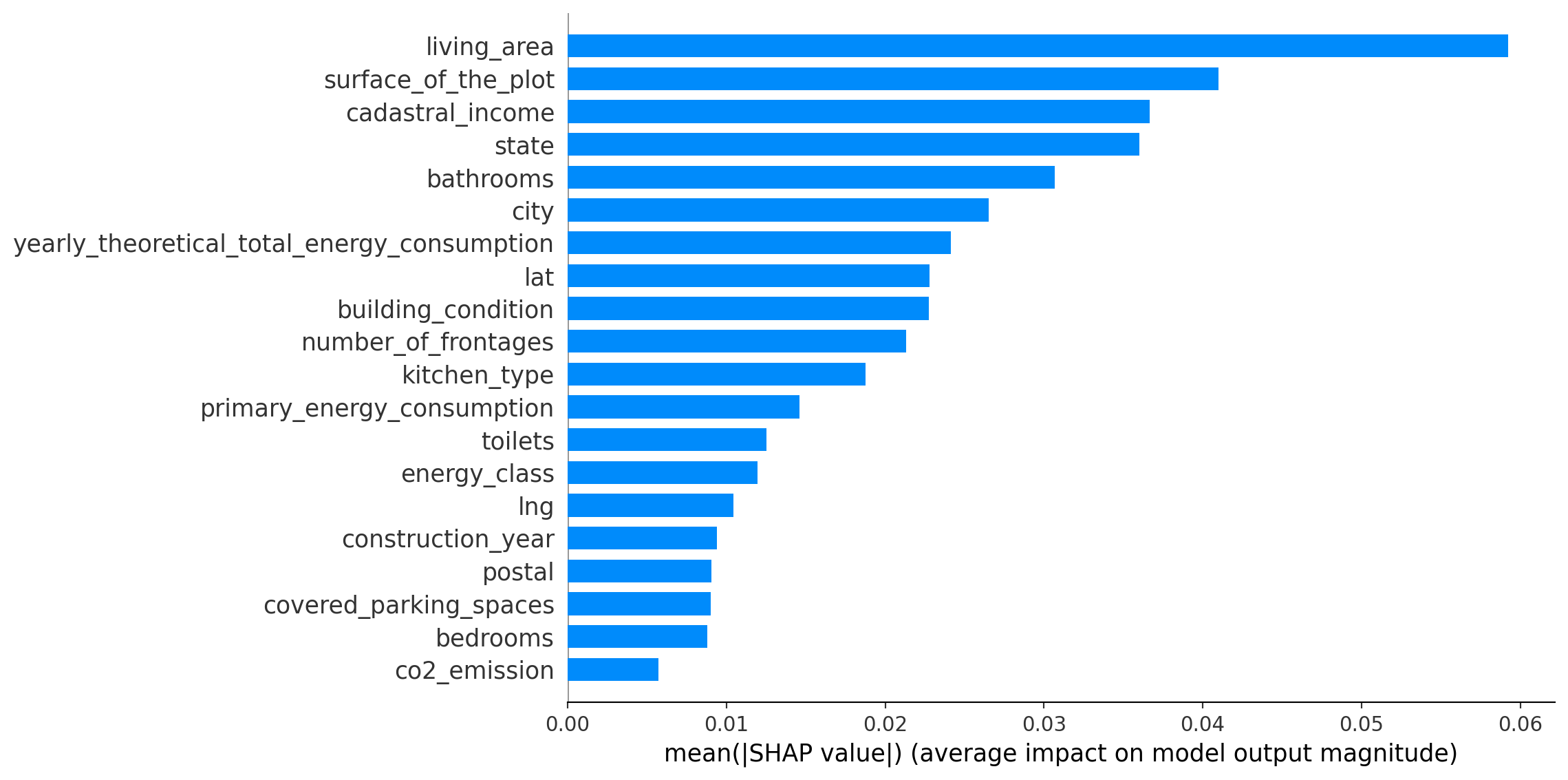
In this phase, our primary focus will involve computing SHAP values and then creating visualizations, such as bar plots and beeswarm plots, to illustrate feature importance and interactionss.
The summary plot at Figure 2 provides a clear depiction of feature importance within the model. The outcomes reveal that “Living area,” “Surface of the plot,” and “Cadastral income” emerge as pivotal factors in influencing the model’s predictions. These features prominently contribute to determining the model’s results.
Figure 2: Assessing Feature Importance using bar plot
The beeswarm plot (Figure 3) can be best understood through the following breakdown:
The Y-axis arranges the feature names based on their importance, with the most influential features placed at the top.
The X-axis displays the SHAP value, representing the impact of each feature on the model’s output. Features on the right side of the plot exhibit a stronger impact, while those on the left possess a weaker influence.
Moreover: - Each point’s color on the plot signifies the respective feature’s value for that specific data point. Red indicates high values, while blue represents low values. - Every individual point on the plot corresponds to a particular row from the original dataset. Collectively, these points illustrate how different data points and their associated feature values contribute to the model’s predictions, especially concerning feature importance.
Upon examining the “living area” feature, you’ll notice it predominantly displays a high positive SHAP value. This suggests that a larger living area tends to have a positive effect on the output, which in this context is the price. Conversely, higher values of “primary energy consumption” are associated with a negative impact on the price, reflected by their negative SHAP values.
Consideration of the spread of SHAP values and their relation to predictive power is important. A wider spread or a denser distribution of data points implies greater variability or a more significant influence on the model’s predictions. This insight allows us to evaluate the significance of features regarding their contribution to the model’s overall output.
This context clarifies why “living area” holds greater importance compared to “CO2 emission.” The broader impact and higher variability of the “living area” feature in influencing the model’s predictions make it a more crucial determinant of the output, thus carrying more weight in the model’s decision-making process.rtance.
Code
shap.summary_plot(shap_values, tr_X)
No data for colormapping provided via 'c'. Parameters 'vmin', 'vmax' will be ignored
Figure 3: Assessing Feature Importance using beeswarm plot
Let’s examine the ranking or order of feature importances derived from both Gini impurity and SHAP values to understand how they compare and whether they yield similar or differing insights. As you can see from the table below, they are fairly similar.
Recursive feature elimination based on SHAP values
Next, we’ll work on the initial feature elimination process based on SHAP values using CatBoost’s select_features method. Although a rich set of features can be advantageous, the quest for model interpretability prompts us to consider the need for a streamlined feature set.
Our objective here is to remove features that have minimal impact on the final predictive output, retaining only the most influential ones. This action streamlines our model, enhancing its interpretability and making it easier to comprehend the factors driving its predictions.s.
Through Recursive Feature Elimination, we’ve successfully decreased the number of features from an initial count of 49 to a more concise set of 17, up to and including the “bedrooms” feature. This reduction in features hasn’t notably affected our model’s performance, enabling us to retain a comparable level of predictive accuracy. This streamlined dataset enhances the model’s simplicity and interpretability without compromising its effectiveness.
That’s it for now. In the next post, our focus will be on identifying potential outliers within our dataset. Additionally, we’ll delve into several further feature engineering steps aimed at bolstering our model’s performanceFor this, we will useof cross-validation, ensuring the robustness and reliability of our modes. Looking forward to the next steps!
Source Code
---title: 'Predicting Belgian Real Estate Prices: Part 5: Initial feature selection'author: Adam Cseresznyedate: '2023-11-07'categories: - Predicting Belgian Real Estate Pricesjupyter: python3toc: trueformat: html: code-fold: true code-tools: true---{fig-align="center" width=50%}In Part 4, we looked into some crucial sample pre-processing steps before modeling, establishing the required pipeline for data processing, evaluating various algorithms, and ultimately identifying an appropriate baseline model, that is CatBoost. As we proceed to Part 5, our focus will be on assessing the significance of features in the initial scraped dataset. We'll achieve this by employing the `feature_importances_` method of CatBoostRegressor and analyzing SHAP values. Additionally, we'll systematically eliminate features showing lower importance or predictive capability. Excited to delve into this phase!::: {.callout-note}You can access the project's app through its [Streamlit website](https://belgian-house-price-predictor.streamlit.app/).:::# Import data```{python}#| editable: true#| slideshow: {slide_type: ''}#| tags: []from pathlib import Pathimport catboostimport numpy as npimport pandas as pdimport shapfrom data import pre_process, utilsfrom IPython.display import clear_outputfrom lets_plot import*from lets_plot.mapping import as_discretefrom models import train_modelfrom sklearn import metrics, model_selectionfrom tqdm import tqdmLetsPlot.setup_html()```# Prepare dataframe before modelling## Read in dataframe```{python}df = pd.read_parquet( utils.Configuration.INTERIM_DATA_PATH.joinpath("2023-10-01_Processed_dataset_for_NB_use.parquet.gzip" ))```## Train-test splitOur initial step involves executing a train-test split. This process divides the data into two distinct sets: a training set and a testing set. The training set is employed for model training, while the testing set is exclusively reserved for model evaluation. This methodology allows models to be trained on the training set and then assessed for accuracy using the unseen testing set. Ultimately, this approach enables an unbiased evaluation of our model's performance, utilizing the test set that remained untouched during the model training phase.```{python}train, test = model_selection.train_test_split( df, test_size=0.2, random_state=utils.Configuration.seed)print(f"Shape of train: {train.shape}")print(f"Shape of test: {test.shape}")```## Preprocess dataframe for modellingOur first step entails removing features that lack informative value for our model, including 'external_reference', 'ad_url', 'day_of_retrieval', 'website', 'reference_number_of_the_epc_report', and 'housenumber'. After this, we'll proceed to apply a log transformation to our target variable. Furthermore, we'll address missing values in categorical features by replacing them with the label "missing value." This step is crucial as CatBoost can handle missing values in numerical columns, but for categorical missing values, user intervention is needed.```{python}processed_train = ( train.reset_index(drop=True) .assign(price=lambda df: np.log10(df.price)) # Log transformation of 'price' column .drop(columns=utils.Configuration.features_to_drop))# This step is needed since catboost cannot handle missing values when feature is categoricalfor col in processed_train.columns:if processed_train[col].dtype.name in ("bool", "object", "category"): processed_train[col] = processed_train[col].fillna("missing value")processed_train.shape```# Inspect feature importanceTo evaluate feature importance, we're utilizing two methods: the `feature_importances_` attribute in CatBoost and SHAP values from the SHAP library. To begin examining feature importances, we'll initiate model training. This involves further partitioning the training set, reserving a portion for CatBoost training (validation dataset). This segmentation allows us to stop the training process when overfitting emerges. Preventing overfitting is crucial, as it ensures we don't work with an overly biased model. Additionally, if overfitting occurs, stopping training earlier helps conserve time and resources.```{python}features = processed_train.columns[~processed_train.columns.str.contains("price")]numerical_features = processed_train.select_dtypes("number").columns.to_list()categorical_features = processed_train.select_dtypes("object").columns.to_list()train_FS, validation_FS = model_selection.train_test_split( processed_train, test_size=0.2, random_state=utils.Configuration.seed)# Get target variablestr_y = train_FS[utils.Configuration.target_col]val_y = validation_FS[utils.Configuration.target_col]# Get feature matricestr_X = train_FS.loc[:, features]val_X = validation_FS.loc[:, features]print(f"Train dataset shape: {tr_X.shape}{tr_y.shape}")print(f"Validation dataset shape: {val_X.shape}{val_y.shape}")``````{python}train_dataset = catboost.Pool(tr_X, tr_y, cat_features=categorical_features)validation_dataset = catboost.Pool(val_X, val_y, cat_features=categorical_features)```As you can see below, the training loss steadily decreases, but the validation loss reaches a plateau. Thanks to the validation dataset, we can halt the training well before the initially set 2000 iterations. This early cessation is crucial for preventing overfitting and ensures a more balanced and effective model.```{python}model = catboost.CatBoostRegressor( iterations=2000, random_seed=utils.Configuration.seed, loss_function="RMSE",)model.fit( train_dataset, eval_set=[validation_dataset], early_stopping_rounds=20, use_best_model=True, verbose=2000, plot=True,)```According to our trained CatBoost model, the most significant feature in our dataset is the living_area, followed by cadastre_income and latitude. To validate and compare these findings, we'll examine the SHAP values to understand how they align or differ from the feature importances provided by the model.```{python}#| fig-cap: Assessing Feature Importance#| label: fig-fig1( pd.concat( [pd.Series(model.feature_names_), pd.Series(model.feature_importances_)], axis=1 ) .sort_values(by=1, ascending=False) .rename(columns={0: "name", 1: "importance"}) .reset_index(drop=True) .pipe(lambda df: ggplot(df, aes("name", "importance"))+ geom_bar(stat="identity")+ labs( title="Assessing Feature Importance", subtitle=""" based on the feature_importances_ attribute """, x="", y="Feature Importance", caption="https://www.immoweb.be/", )+ theme( plot_subtitle=element_text( size=12, face="italic" ), # Customize subtitle appearance plot_title=element_text(size=15, face="bold"), # Customize title appearance )+ ggsize(800, 600) ))```# SHAPSHAP (SHapley Additive exPlanations) values offer a method to elucidate the predictions made by any machine learning model. These values leverage a game-theoretic approach to quantify the contribution of each "player" (feature) to the final prediction. In the realm of machine learning, SHAP values assign an importance value to each feature, delineating its contribution to the model's output.SHAP values provide detailed insights into how each feature influences individual predictions, their relative significance in comparison to one another, and the model's reliance on interactions between features. This comprehensive perspective enables a deeper understanding of the factors that drive the model's decision-making process.In this phase, our primary focus will involve computing SHAP values and then creating visualizations, such as bar plots and beeswarm plots, to illustrate feature importance and interactionss.```{python}shap.initjs()explainer = shap.TreeExplainer(model)shap_values = explainer.shap_values( catboost.Pool(tr_X, tr_y, cat_features=categorical_features))```The summary plot at @fig-fig2 provides a clear depiction of feature importance within the model. The outcomes reveal that "Living area," "Surface of the plot," and "Cadastral income" emerge as pivotal factors in influencing the model's predictions. These features prominently contribute to determining the model's results.```{python}#| fig-cap: Assessing Feature Importance using bar plot#| label: fig-fig2shap.summary_plot(shap_values, tr_X, plot_type="bar", plot_size=[12, 6])```The beeswarm plot (@fig-fig3) can be best understood through the following breakdown:- The Y-axis arranges the feature names based on their importance, with the most influential features placed at the top.- The X-axis displays the SHAP value, representing the impact of each feature on the model's output. Features on the right side of the plot exhibit a stronger impact, while those on the left possess a weaker influence.Moreover:- Each point's color on the plot signifies the respective feature's value for that specific data point. Red indicates high values, while blue represents low values.- Every individual point on the plot corresponds to a particular row from the original dataset. Collectively, these points illustrate how different data points and their associated feature values contribute to the model's predictions, especially concerning feature importance.Upon examining the "living area" feature, you'll notice it predominantly displays a high positive SHAP value. This suggests that a larger living area tends to have a positive effect on the output, which in this context is the price. Conversely, higher values of "primary energy consumption" are associated with a negative impact on the price, reflected by their negative SHAP values.Consideration of the spread of SHAP values and their relation to predictive power is important. A wider spread or a denser distribution of data points implies greater variability or a more significant influence on the model's predictions. This insight allows us to evaluate the significance of features regarding their contribution to the model's overall output.This context clarifies why "living area" holds greater importance compared to "CO2 emission." The broader impact and higher variability of the "living area" feature in influencing the model's predictions make it a more crucial determinant of the output, thus carrying more weight in the model's decision-making process.rtance.```{python}#| fig-cap: Assessing Feature Importance using beeswarm plot#| label: fig-fig3shap.summary_plot(shap_values, tr_X)```Let's examine the ranking or order of feature importances derived from both Gini impurity and SHAP values to understand how they compare and whether they yield similar or differing insights. As you can see from the table below, they are fairly similar.```{python}catboost_feature_importance = ( pd.concat( [pd.Series(model.feature_names_), pd.Series(model.feature_importances_)], axis=1 ) .sort_values(by=1) .rename(columns={0: "catboost_name", 1: "importance"}) .reset_index(drop=True))``````{python}shap_feature_importance = ( pd.DataFrame(shap_values, columns=tr_X.columns) .abs() .mean() .sort_values() .reset_index() .rename(columns={"index": "shap_name", 0: "shap"}))``````{python}pd.concat( [ catboost_feature_importance.drop(columns="importance"), shap_feature_importance.drop(columns="shap"), ], axis=1,)```# Recursive feature elimination based on SHAP valuesNext, we'll work on the initial feature elimination process based on SHAP values using CatBoost's `select_features` method. Although a rich set of features can be advantageous, the quest for model interpretability prompts us to consider the need for a streamlined feature set.Our objective here is to remove features that have minimal impact on the final predictive output, retaining only the most influential ones. This action streamlines our model, enhancing its interpretability and making it easier to comprehend the factors driving its predictions.s.```{python}regressor = catboost.CatBoostRegressor( iterations=1000, cat_features=categorical_features, random_seed=utils.Configuration.seed, loss_function="RMSE",)rfe_dict = regressor.select_features( algorithm="RecursiveByShapValues", shap_calc_type="Exact", X=tr_X, y=tr_y, eval_set=(val_X, val_y), features_for_select="0-48", num_features_to_select=1, steps=10, verbose=250, train_final_model=False, plot=True,)```Through Recursive Feature Elimination, we've successfully decreased the number of features from an initial count of 49 to a more concise set of 17, up to and including the "bedrooms" feature. This reduction in features hasn't notably affected our model's performance, enabling us to retain a comparable level of predictive accuracy. This streamlined dataset enhances the model's simplicity and interpretability without compromising its effectiveness.```{python}features_to_keep = ( rfe_dict["eliminated_features_names"][33:] + rfe_dict["selected_features_names"])print(features_to_keep)```That's it for now. In the next post, our focus will be on identifying potential outliers within our dataset. Additionally, we'll delve into several further feature engineering steps aimed at bolstering our model's performanceFor this, we will useof cross-validation, ensuring the robustness and reliability of our modes. Looking forward to the next steps!